The sampSurf Package: Sampling Surface Simulation
Overview of the sampSurf package
The
In general we are interested in determining the properties of various sampling methods
mentioned above when applied to fixed objects such as standing trees or down logs. The
There are several vignettes associated with the package that provide detailed explanation
and examples of the design and use of the various components. A good place to start is
with The sampSurf Package Overview vignette, which provides an overview of the
class structure, etc. The vignettes are all available from the package index help page
once the package has been installed and loaded using
Down Logs
- Fixed-area plots:
stand-up, sausage, andchainsaw protocols - Point-relascope sampling
- Perpendicular distance sampling (PDS)
- Omnibus PDS
- Distance-limited PDS: canonical, hybrid and omnibus protocols
- Distance-limited sampling: traditional and crude Monte Carlo protocols
- Fixed-area plots:
Standing Trees
- Fixed-area plots
- Horizontal point sampling
- Horizontal point sampling with Monte Carlo subsampling (see below)
- Horizontal line sampling
- Critical height sampling
- Importance critical height sampling
- Antithetic importance critical height sampling
- Paired antithetic importance critical height sampling
A recent addition to the package (in version 0.7-0) is the ability to sample down logs or standing trees for volume using Monte Carlo methods. These include crude Monte Carlo, importance sampling, control variate sampling, and antithetic versions of each. These are not areal methods, and apply directly to the stem objects themselves, so stem-based simulations can be conducted independently of an areal method. However, they can also be added to any areal method for a two-stage approach. For example, this has been incorporated in horizontal point sampling for standing trees.
Furthermore, as of version 0.7-2, the mirage method is available in addition to buffering
for correction of boundary slopover. As in the buffer method, mirage correction is
accomplished by running a simulation on a special mirage
For more information on how each of these sampling and boundary correction methods is
implemented within
sampSurf installation
On the project pages, you will note that you can install the package directly from R-Forge
using…
and can include the
Optional…
The above should do it, while getting the correct stable releases from CRAN prior to
installing
Enabling the R help system
One other thing that some R users may not be getting the full advantage of is the html
help system. This really should be set up to work correctly in your .Rprofile
file to get help via your web browser, using the local help file installation for each
package (not just .Rprofile…
That should do it on Linux, I have not tested this on other platforms, but it probably
will work. Now when you do something like
rgl Installation
On Linux, the freeglut-devel and libpng-devel which could be installed
with yum prior to installing
sampSurf package vignettes
As noted above, there are a number of package vignettes distributed with the package itself. These can also be downloaded here from the R-Forge versions if desired…
-
Getting Started with Package
sampSurf -
The
sampSurf Package Overview -
The
ArealSampling Class -
The
Stem Class -
The
Tract Class -
The
InclusionZone Class -
The
InclusionZoneGrid Class -
The
sampSurf Class
In addition, I have decided to remove some of the vignettes from the actual package structure itself because of the amount of space they consume, or the fact that they may be of limited interest to most users. Thus, the vignettes below are only available here at R-Forge…
-
sampSurf : Sampling Surface Simulation for Areal Sampling Designs in R -
monte : When is n Sufficiently Large? -
Monte Carlo Sampling Methods in
sampSurf -
The Mirage Method in
sampSurf -
Extending the
sampSurf Package
Perhaps the most helpful introduction to
sampSurf examples
Here we present some very simple examples illustrating how to use a few of the main
functions in the
In general, there are two main ways to create a sampling surface: (1) simple, usually "one-off" construction, or (2) progressive, by constructing intermediate elements that can be re-used for comparison of methods, etc. Both will be demonstrated below.
Simple sampling surface construction
The first example shows how to create a sampling surface "on-the-fly," as it were, by
hiding the intermediate steps used in building the surface. The only exception is that we
always need some form of
The first component that is always required for a completed sampling surface is a
R> require(sampSurf)
R> tract.m = Tract(c(x = 71, y = 71), cellSize = 0.5)     #meters
R> buffTract.m = bufferedTract(bufferWidth = 10, tract.m)
In the above example, we have first made a
Next, simply run the
R> sausageLen.ss = sampSurf(20, tract = buffTract.m, iZone = 'sausageIZ',
+                          plotRadius = 3, estimate = 'Length',
+                          buttDiams = c(20, 50), logLens = c(2, 8))
Number of logs in collection = 20
Heaping log: 1,2,3,4,5,6,7,8,9,10,11,12,13,14,15,16,17,18,19,20,
R> plot(sausageLen.ss, useImage = FALSE)
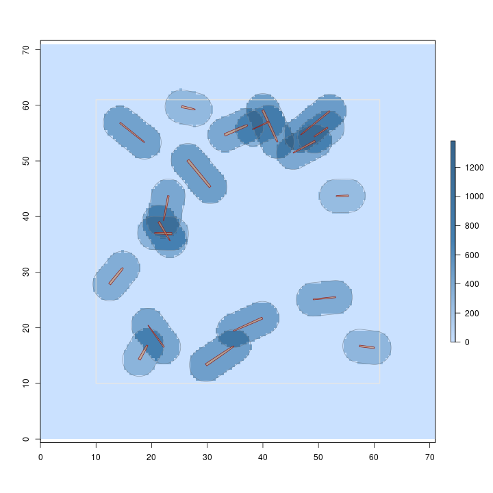
Notice that you can specify the default log dimensions (e.g.,
A summary of the object is often useful…
R> sausageLen.ss
Object of class: sampSurf
------------------------------------------------------------
sampling surface object
------------------------------------------------------------

Inclusion zone objects: sausageIZ
Estimate: Length
Number of logs = 20

------------------------------------------------------------
object of class Tract
------------------------------------------------------------
Measurement units = metric
Area in square meters = 5041 (0.5041 hectares)

class       : bufferedTract
dimensions  : 142, 142, 20164  (nrow, ncol, ncell)
resolution  : 0.5, 0.5  (x, y)
extent      : 0, 71, 0, 71  (xmin, xmax, ymin, ymax)
coord. ref. : NA
data source : in memory
names       : surf
values      : 0, 1380.7419  (min, max)

Buffer width =  10
R> summary(sausageLen.ss)
Object of class: sampSurf
------------------------------------------------------------
sampling surface object
------------------------------------------------------------

Inclusion zone objects: sausageIZ
Measurement units = metric
Number of logs = 20
True log volume = 6.1546085 cubic meters
True log length = 86.33 meters
True log surface area = 77.289279 square meters
True log coverage area = 24.565998 square meters
True log biomass = NA
True log carbon = NA

Estimate attribute: Length
Surface statistics...
  mean = 86.11307
  bias = -0.21693013
  bias percent = -0.25128012
  sum = 1736383.9
  var = 45264.698
  st. dev. = 212.75502
  cv % = 247.06472
  surface max = 1380.7419
  total # grid cells = 20164
  grid cell resolution (x & y) = 0.5 meters
  # of background cells (zero) = 16741
  # of inclusion zone cells = 3423
Printing the object in the first line, displays the specification on the
internal
We can also display the surface nicely using the
R> require(rgl)
R> plot3D(sausageLen.ss)
R> par3d(zoom = 0.8)
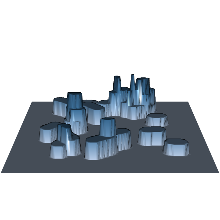
Note that sampling for log length under the sausage sampling protocol of fixed-area plot sampling yields a constant height surface for each log, which varies between logs. This method is a probability proportional to length estimation method, and normally the heights would be constant for all logs under such a design. But sausage sampling is a little different in this respect because of the way the inclusion area is determined.
Detailed sampling surface construction
In this section we will look at elaborating on what was done in the previous section by
showing how a sampling surface can be built by creating most of the intermediate objects
"by hand." (I say "most" here because
- Create a
Tract object. - Create a population of synthetic stems in the form of logs or trees.
- If need be, create an
ArealSampling object with the specifications for the method. - Combine the stem population and the sampling method in the last two steps
and form the population of
InclusionZone objects. - Create the sampling surface from the collection in the previous step.
We will use the
R> dLogs = downLogs(25, buffTract.m, buttDiams = c(25, 50), logLens = c(5, 10))
R> dLogs
Object of class: downLogs
------------------------------------------------------------

------------------------------------------------------------
Container class object...
  Units of measurement:  metric

  Encapulating bounding box...
        min       max
x 7.4339276 62.758264
y 8.7174424 62.270595

  There are 25 logs in the population
  Population log volume =  14.230931 cubic meters
  Population log surface area =  174.73371 square meters
  Population log coverage area =  55.585258 square meters
  Average volume/log =  0.56923725 cubic meters
  Average surface area/log =  6.9893486 square meters
  Average coverage area/log =  2.2234103 square meters
  Average length/log =  7.3228 meters
(**All statistics exclude NAs)
R> plot(buffTract.m, gridColor = 'grey70')
R> plot(dLogs, add = TRUE)
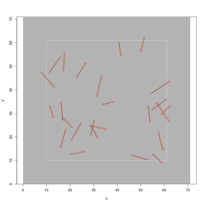
We created a population of rather long, and large-diameter logs so they display nicely on
the plot (remember, this is a metric example, and the
Next, since we know we want to use pds, we need to create an object that contains the information about that sampling method in the form of design parameters for the distance limit. This is most easily done in terms of a "Kpds factor" for the method…
R> pds.m = perpendicularDistance(50, description = 'PDS parameters')
R> pds.m
Object of class: perpendicularDistance
------------------------------------------------------------
PDS parameters
------------------------------------------------------------

ArealSampling...
  units of measurement:  metric

perpendicularDistance...
  kPDS factor = 50 per meter [or dimensionless] for volume [surface/coverage area]
  volume [surface/coverage area] factor = 100 cubic meters [square meters] per hectare
The default is for metric units as we can see in the object summary. The associated
volume, surface and coverage areas are determined for this particular
Kpds factor and are also shown in the summary. I don't want
to get into the structure of the package classes too much at this point, but the summary
shows that the
The next step is to combine the collection of down logs and the appropriate sampling
method parameters (the last two objects created above) and make the inclusion zones for
each log. In the end, what we want is a collection of inclusion zones, one for each log,
to match the
R> dLogs.izs = downLogIZs(dLogs, iZone = 'perpendicularDistanceIZ', pds = pds.m,
+                        pdsType = 'volume',
+                        description = 'pds inclusion zones for dLogs')
R> dLogs.izs
Container object of class: downLogIZs
------------------------------------------------------------
pds inclusion zones for dLogs
------------------------------------------------------------
There are 25 inclusion zones in the population
Inclusion zones are of class: perpendicularDistanceIZ
Units of measurement:  metric
Summary of inclusion zone areas in square meters...
      Min.    1st Qu.     Median       Mean    3rd Qu.       Max.
 24.594249  39.287022  52.811780  56.923725  73.104563 140.605338
       var       SDev
607.335010  24.644168

Encapulating bounding box...
        min       max
x 6.3594000 70.025991
y 5.0145724 63.960017
R> plot(buffTract.m, gridColor = 'grey70')
R> plot(dLogs.izs, add = TRUE)
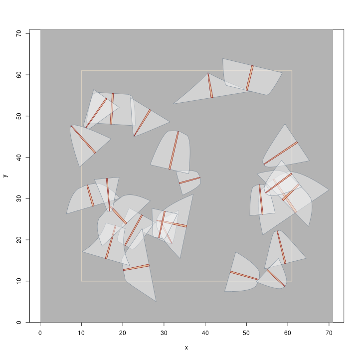
Note that the
R> dLogs.ss = sampSurf(dLogs.izs, buffTract.m)
Number of logs in collection = 25
Heaping log: 1,2,3,4,5,6,7,8,9,10,11,12,13,14,15,16,17,18,19,20,21,22,23,24,25,
R> summary(dLogs.ss)
Object of class: sampSurf
------------------------------------------------------------
sampling surface object
------------------------------------------------------------

Inclusion zone objects: perpendicularDistanceIZ (with PP to: volume)
Measurement units = metric
Number of logs = 25
True log volume = 14.230931 cubic meters
True log length = 183.07 meters
True log surface area = 174.73371 square meters
True log coverage area = 55.585258 square meters
True log biomass = NA
True log carbon = NA

Estimate attribute: volume
Surface statistics...
  mean = 14.21
  bias = -0.020931233
  bias percent = -0.14708266
  sum = 286530.44
  var = 825.22058
  st. dev. = 28.726653
  cv % = 202.15801
  surface max = 151.23
  total # grid cells = 20164
  grid cell resolution (x & y) = 0.5 meters
  # of background cells (zero) = 15534
  # of inclusion zone cells = 4630
R> plot(dLogs.ss, useImage = FALSE)
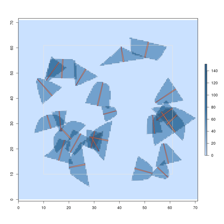
Note in the summary that the method is unbiased. And, as in the first example, we can
visualize the surface using
R> require(rgl)
R> plot3D(dLogs.ss)
R> par3d(zoom = 0.8)
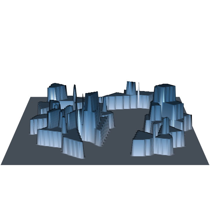
Because we are sampling with probability proportional to volume, and estimating volume, the volume estimate for each log is the same and it gets spread evenly over its inclusion zone under pds. Also, since each log accounts for the same estimate (the volume factor), we get an even stair-step "heaping" of the surface where the inclusion zones intersect. This is the more normal case when you are sampling to estimate the "design attribute" that the method is optimized in terms of; the sausage protocol above is an exception to this rule.
A final example
In the previous examples we have ignored standing trees and English units. Here we will
rectify this. The steps presented below are the same as those outlined in the previous
section, except they are applied to standing trees (and of course, the vignettes have much
more detail on each step). You can look at
(e.g.,
R> tract.e = Tract(c(x = 208, y = 209), units = 'English', cellSize = 1) #feet here
R> buffTract.e = bufferedTract(bufferWidth = 30, tract.e)
R> sTrees = standingTrees(20, buffTract.e, dbhs = c(6, 15), heights = c(30, 50),
+                        units = 'English')
R> aGauge = angleGauge(baf = 20, units = 'English')
R> sTrees.izs = standingTreeIZs(sTrees, iZone = 'horizontalPointIZ',
+                              angleGauge = aGauge)
R> hps.ss = sampSurf(sTrees.izs, buffTract.e, estimate = 'Density')
Number of trees in collection = 20
Heaping tree: 1,2,3,4,5,6,7,8,9,10,11,12,13,14,15,16,17,18,19,20,
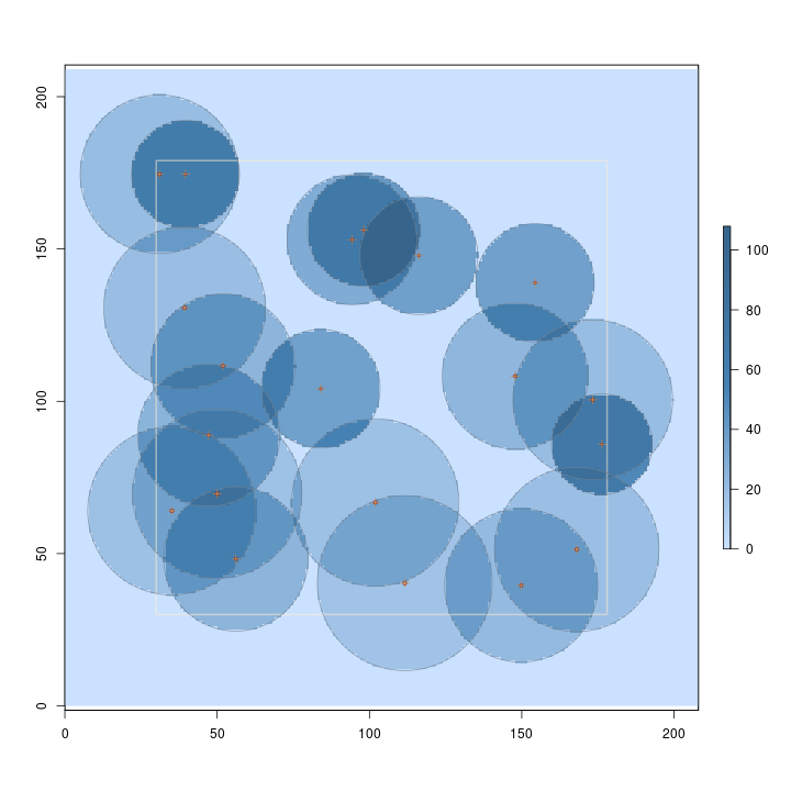
R> plot(hps.ss, useImage = FALSE)
R> require(rgl)
R> plot3D(hps.ss)
R> par3d(zoom = 0.8)
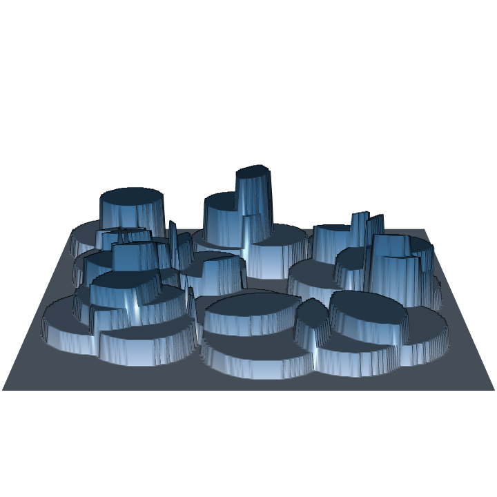
Note in the figures that larger trees represent fewer trees per acre, and thus have lower surface height than smaller trees. Some sampling methods (or protocols for a given method) even have variable height surfaces within individual inclusion zones for each stem, perhaps you'll stumble across these in the use of this package.
Summary
The examples presented assume some knowledge of the subject area with respect to areal
sampling methods. Hopefully one can get an idea of what is involved in using the package
and some uses it might be put to by comparing different (or new) methods on the sample
stem populations. The vignettes provide much more detail and both they and the help pages
have references to some of the more recent papers on both the sampling methods and the
sampling surface concept. Please let me know if you've found
